Enterprise AI Model Metrics: Part 2
To drive business value through the use of enterprise AI models, it is essential that those models are trained and tuned to optimize the right metrics. A failure to use the right metrics to evaluate AI models could lead to a failure in realizing the maximum business value possible from AI-driven applications. This article is the second in a two-part series on binary classification metrics, through which I seek to share insights that can help identify the right metrics to optimize for different enterprise AI applications.
The focus of this article is on understanding metrics that can be used to compare multiple AI models using a validation dataset, and to help decide which of those models should be selected to deliver maximum business value. The choice of metric with which to evaluate an AI model depends on the cost of each decision that the model could make and on the extent of imbalance in the distribution of classes of data in the dataset. This article is aimed at helping you avoid some mistakes that I have seen AI practitioners and business leaders make when choosing metrics, using them for model evaluation, and drawing conclusions from them to make business decisions.
The metrics that we will cover in this article are the ROC curve, precision, recall, and the F1 score. Those metrics build upon the definitions described in Part 1 of this series.
Varying thresholds on the AI model score
An AI model makes a decision about whether a certain case is to be predicted as positive or negative based on whether the probability that it belongs to that class (positive or negative) surpasses a given threshold. The threshold is either learned by the model or tuned via a hyperparameter to the model.
Let’s take an example of an AI model that produces a risk score for whether an industrial systems component is currently faulty. That is exactly the type of model that most C3 AI Reliability applications use. For the sake of being generic, let us refer to that score as the AI score. There are many ways to generate such a score using either supervised or unsupervised learning methods.
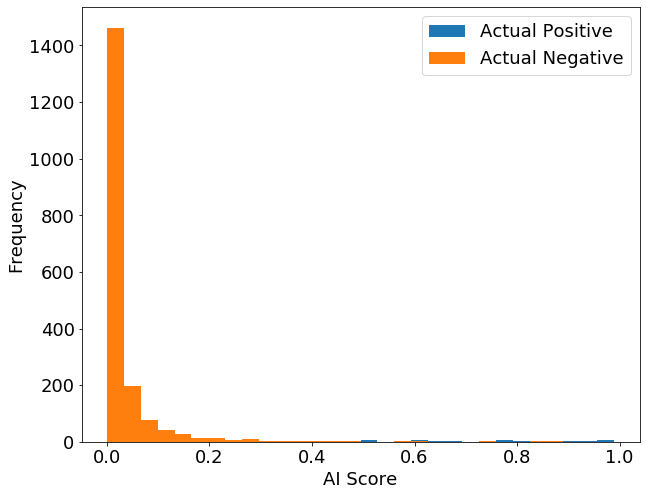
The following histogram captures a typical distribution of positive and negative samples, as scored by an AI model. In this example, the AI model tries to give negative cases low scores and positive cases high scores. Because the vast majority of actual negatives were given a low score, we know that the model is doing a good job on negative cases. It may be hard to see, but there are a few positive cases (blue bars) in the bottom right of the plot which were given a relatively high score by the AI model.
Let’s collapse the vertical axis of the above histogram and view the actual positives and negatives in a single dimension.
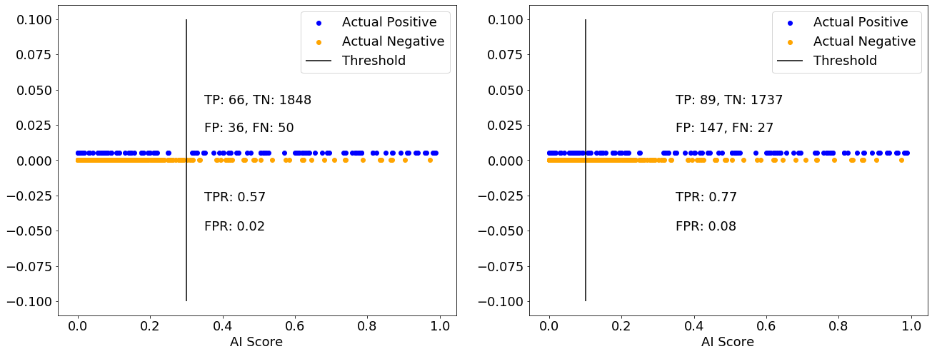
The AI model will flag a case as positive if the AI score is greater than a threshold. The threshold is set at 0.3 in the figure above on the left, and at 0.1 in the figure on the right. The TP count is the number of actual positives (blue dots) to the right of the threshold line, and that increases as you decrease the threshold. However, the FP count – the number of actual negatives (orange dots) to the right of the threshold line – also increases. In the above example, the actual positives and actual negatives are interspersed. Therefore, there is no choice of threshold that will produce zero FPs and FNs at the same time. As a result, the model will always be confused; the degree of confusion can be controlled by the threshold.
In a different example, it is possible, though unlikely, that a threshold can be found that separates the cases into actual positives and actual negatives (imagine a figure similar to the above in which all blue dots are to the right of all orange dots). In that scenario, the AI model is not confused (as explained in Part 1 of this article). Whether or not it is possible to find such a threshold depends on how distinguishable positive cases are from negative cases in the dataset. In most datasets, there are at least a few cases where positives and negatives are difficult to distinguish, and that leads to some confusion.
Depending on where the threshold is set on the AI score, the AI model will achieve a different true positive rate (TPR) and false positive rate (FPR) as shown in the example plot below.
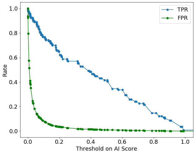
This plot illustrates the trade-off between TPRs and FPRs.
If we set the threshold on the AI score at 0, then the AI model will flag all cases as positive. It will then achieve a TPR of 100 percent, but also an FPR of 100 percent. So, if you meet a data scientist who claims to have a model that provides a TPR of 100 percent, you must ask for the FPR. If the model has an FPR of 100 percent, it is probably useless.
Similarly, if we set the threshold on the AI score at 1, then the AI model will flag all cases as negative. That will achieve an ideal FPR of 0 percent, but a poor TPR of 0 percent.
Note that Scikit-Learn, a popular Python library used for machine learning, assumes that the threshold to be used in the AI model’s “predict” function is 0.5 by default. Notice in the above plot that 0.5 is far from optimal (somewhere around 0.1 would have achieved a much higher TPR for a similar FPR). Using the ‘predict’ function without considering other thresholds is a common mistake made by AI practitioners. There are multiple approaches (both good and bad) to identify the best threshold, and we will discuss some of those next.
The Receiver Operating Characteristic (ROC) Curve
The ROC curve is simply a scatter plot of TPR and FPR values for different choices of thresholds (you’d be surprised how often candidates I interview are unable to correctly name the axes, usually confusing them for TP vs. FP instead of TPR vs. FPR).
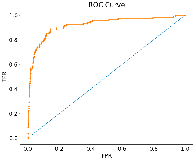
The ROC curve captures the trade-off between TPR and FPR without explicitly plotting the value of the thresholds anywhere. The area under the ROC curve, often referred to as the AUC, ranges from 0 to 1. If there is no confusion, the AUC is 1. The AUC is an indicator of how well the AI model is able to discriminate a positive case from a negative case.
Let’s look at a trickier question that we have (in the past) used as part of our data science interview process. In which of the below three examples is the AI model least capable of being discriminative?

Candidates who guessed AUC = 0.08 as the answer did not make it to the next round of our data science interview. That is because a model with AUC = 0.08 has the same discriminative ability as a model with AUC = 0.92. It is predicting the wrong class so consistently that if you swapped “positive” predictions for “negative” predictions (and vice versa), you would end up with a helpful model (AUC = 0.92). The model with AUC = 0.5 is the least useful model as it is equivalent to taking a uniform, random guess.
The ROC curve/AUC are popular ways to determine a suitable threshold for detecting positive cases. But in my opinion, they are overused both in academic literature and industry (that opinion is supported in this article by an independent blogger and references therein). While they work well in most cases, they are not suitable for use with highly imbalanced datasets where the ratio of true positives to false positives is important.
Let’s take an example of a model that achieves the following:
In the above example, the TPR = 90% and FPR = 1%. That seems like a really good model, and if several thresholds were to produce similar values, the AUC is likely to be close to 1. However, we have more than 20 false positives for each true positive. Think of what that could mean if that model were predicting that a patient is positive for COVID-19. We would know that the model has a less than one in 20 chance of being right, and that makes the model unreliable. So ROC/AUC would indicate a good model, but we know that’s not true for this use case.
The main issue with using ROC/AUC for imbalanced datasets is that it rewards true negatives, which we don’t want when the total number of negatives far exceeds the total number of positives. That is because the value of FPR can be small if the number of true negatives is large compared to the number of false positives (refer back to the formula).
AI practitioners get around the ROC/AUC pitfall most often by doing one of the following:
- Avoid using ROC/AUC altogether in preference to precision and recall (which we will discuss in the next section).
- Incorporate misclassification costs and use cost curves instead of ROC curves.
- Synthetically balance the dataset by oversampling the minority or undersampling the majority.
Because of the weight it places on true negatives, the ROC/AUC is suitable in situations where we may not want sensitivity to class imbalance. If one model is evaluated on different datasets with different levels of class imbalance in them, the ROC/AUC will not vary much between the datasets.
Precision and Recall
Two metrics that avoid true negatives altogether are precision and recall.
We have already seen recall, which is the same as TPR. Notice that unlike TPR and FPR, which occupy different columns of the confusion matrix, precision and recall overlap with TP as the common numerator.
Precision and recall are each important under different circumstances.
- Precision: Important when the cost of false positives outweighs the cost of false negatives. For example: C3 AI Fraud Detection™, a C3 AI Application wherein it costs a lot of money to investigate the fraud, but the amount of revenue recovered from fraudulent consumers may not be as high.
- Recall: Important when the cost of false negatives outweighs the cost of false positives. For example: C3 AI Predictive Maintenance™, a C3 AI Application wherein a false negative indicates a failure that could lead to loss of life and millions of dollars in machine parts.
The precision-recall curve maps the trade-off between precision and recall for different values of thresholds (similar to the ROC curve for TPR and FPR). And like the AUC, the area under the precision-recall curve ranges from 0 to 1. If there is no confusion, that area is equal to 1. The area combines precision and recall into a single metric that can be used for hyperparameter optimization. It also accounts for different choices of thresholds that could lead to different values of precision and recall.
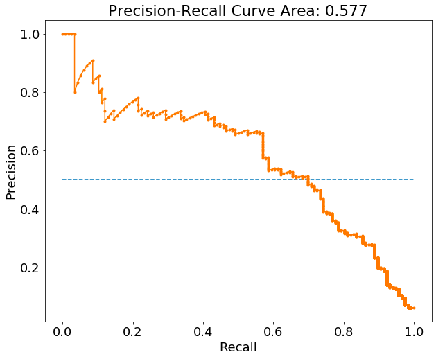
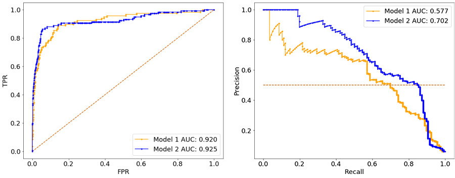
Let’s take an example of how to choose between two different AI models that were trained on the same dataset. The following ROC and precision-recall curves were computed on two hold-out validation sets.
Validation set 1 – 95% negative:
Validation set 2 – 99% negative:
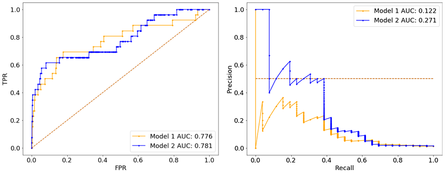
Notice two things from the above illustrations:
- the ROC is very similar between the two models in both validation sets, whereas the precision-recall curves make it clear that Model 2 is more likely to maximize business value in both cases.
- the ROC is more robust to the change in class imbalance than precision-recall curves, which drop by a lot more in the second validation set. However, that hides the fact that the models could have low precision on imbalanced datasets – an important factor to consider before deployment to production.
Fβ Score
The Fβ score is a way to combine the precision and recall formulae into a single metric for a specific choice of threshold. The formula for the Fβ score is as follows:
The most common value for β used by AI practitioners is 1, and the resulting F1 score is often defined as the harmonic mean of precision and recall. The F1 score places an equal weight on precision and recall. For values of β > 1, recall is weighted higher than precision; for values of β < 1, precision is weighted higher than recall.
Unlike the area under the precision-recall curve, the Fβ score is calculated using a single threshold on the AI score. For the same AI model, varying the threshold on the AI score can help find a desirable Fβ score, as shown here:
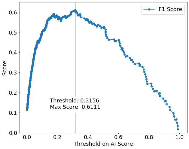
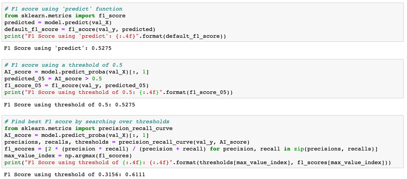
The advantage of using the Fβ score is that it allows you to optimize simultaneously for precision and recall by tuning their weights in a single metric using the β parameter. Having that single metric makes it easier to evaluate a large number of AI model hyperparameters in an automated fashion to produce the most performant model for the AI application. When reporting the Fβ score for each hyperparameter configuration, one must be careful to evaluate all thresholds and report the highest Fβ score that can be obtained using that configuration (as shown in the code snippet below). That evaluation can be done quickly, without requiring the model to be retrained for each threshold, and the threshold corresponding to the highest Fβ score should be saved for use in prediction. Using the ‘predict’ function, which is equivalent to using a threshold of 0.5, will likely lead to suboptimal Fβ values in practice. That can be seen in the above plot. The following example in Python describes the suboptimal and optimal thresholding approaches for computing the F1 score.
The disadvantage of using the Fβ score is that the β parameter may be difficult to obtain or translate from business requirements. A good example of a business requirement from a C3.ai client is the following: the AI model should have a recall of at least 90 percent, and as high of a precision as can be simultaneously achieved. Recall is a satisficing metric while precision is an optimizing metric in that example (it could be the other way around in a different example). AutoML capabilities offered by the C3 AI Application Platfrom™ allow you to define an optimizing metric and one or more satisficing metrics. If you prefer to hand-tune your model, you could use the precision-recall curve to identify a suitable threshold that achieves values for precision and recall that meet the satisficing and optimizing requirements. If you cannot find a threshold that meets the satisficing metric requirement, you could try different algorithms or different ways of feature engineering until you are able to find a model that meets that requirement.
Conclusion
When choosing a metric to select an AI model that maximizes business value, I hope you take four points away from this article:
- ROC/AUC can paint an optimistic view of a model and hide the fact that the model could have low precision on imbalanced datasets. That is because it rewards a high true negative rate by placing an equal importance on positive and negative cases.
- Precision-recall curves are best suited for evaluating AI models on imbalanced datasets because neither precision nor recall reward true negatives.
- Metrics that are dependent on the choice of threshold must be evaluated on all feasible thresholds. Using the default threshold in popular libraries can lead to suboptimal AI performance.
- Although it is convenient to combine precision and recall into a single metric for hyperparameter optimization, it could be more intuitive from a business perspective to treat one of them as a satisficing metric and the other as an optimizing metric.
Stay tuned for future articles that will cover metrics to evaluate enterprise AI models in multi-class classification applications and regression applications.


