

Evaluating Model Performance
Managers implementing machine learning solutions to solve business problems need to understand how to quantify model performance – a critical step that informs model selection and tuning, helps architect the right business processes around the model, and informs decisions about ongoing model maintenance and operations.
Some examples of model performance measures follow.
Classification Performance
As described before, classifiers attempt to predict the probability of discrete outcomes. The correctness of these predictions can be evaluated against ground-truth results. Concepts of true or false positives, precision, recall, F1 scores, and receiver operating characteristic (ROC) curves are key to understanding classifier performance. Each of these concepts is described further in the following sections.
True or False Positives
Consider, for example, a supervised classifier trained to predict customer attrition. Such a classifier may make a prediction about how likely a customer is to ‘unsubscribe’ over a certain period of time.
Evaluating the model’s performance can be summarized by four questions:
- How many customers did the model correctly predict would unsubscribe?
- How many customers did the model correctly predict would not unsubscribe?
- How many customers did the model incorrectly predict would unsubscribe (but did not)?
- How many customers did the model incorrectly predict would not unsubscribe (but did)?
These four questions characterize the fundamental performance metrics of true positives, true negatives, false positives, and false negatives. Figure 15 visually describes this concept.
Attrition predictions made by the model are in the top half of the square. Each prediction is either true (the customer will unsubscribe), or not (the customer will not unsubscribe) – and are therefore true or false positives.
The total number of customer attrition predictions made by the classifier is the number of true positives plus the number of false positives.
There are two other concepts highlighted in the figure. False negatives (bottom left) refer to attrition predictions that should have been made but were not. These represent customers who unsubscribed, but who were not correctly classified. True negatives (bottom right) refer to customers who were correctly classified as remaining (not unsubscribing).

Figure 15 Visual representation of true positives, false positives, true negatives, and false negatives
Precision
Precision refers to the number of true positives divided by the total number of positive predictions – the number of true positives, plus the number of false positives. Precision therefore is an indicator of the quality of a positive prediction made by the model.
Precision is defined as:

In the customer attrition example, precision measures the number of customers that the model correctly predicted would unsubscribe divided by the total number of customers the model predicted would unsubscribe.
Recall
Recall refers to the number of true positives divided by the total number of positive cases in the data set (true positives plus false negatives). Recall is a good indicator of the ability of the model to identify the positive class.
Recall is defined as:

In the customer attrition example, recall measures the ratio of customers that the model correctly predicted would unsubscribe to the total number of customers who actually unsubscribed (whether correctly predicted or not).
While a perfect classifier may achieve 100 percent precision and 100 percent recall, real-world models never do. Models inherently tradeoff between precision and recall; typically the higher the precision, the lower the recall, and vice versa.
In the customer attrition example, a model that is tuned for high precision – each prediction is a high-quality prediction – will usually have a lower recall; in other words, the model will not be able to identify a large portion of customers who will actually unsubscribe.
F1 Score
The F1 score is a single evaluation metric that aims to account for and optimize both precision and recall. It is defined as the harmonic mean between precision and recall. Data scientists use F1 scores to quickly evaluate model performance during model iteration phases by collapsing both precision and recall into this single metric. This helps teams test thousands of experiments simultaneously and identify top-performing models quantitatively.
A model will have a high F1 score if both precision and recall are high. However, a model will have a low F1 score if one factor is low, even if the other is 100 percent.
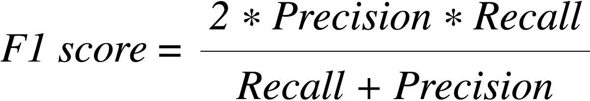
The F1 score is defined as:
Receiver Operating Characteristic (ROC) Curve
Another tool used by data scientists to evaluate model performance is the receiver operating characteristic (ROC) curve. The ROC curve plots the true positive rate (TPR) versus the false positive rate (FPR).
TPR refers to the number of positive cases surfaced as the model makes predictions divided by the total number of positive cases in the data set. This metric is the same as recall.
TPR is defined as:

FPR refers to the number of negative cases that have been surfaced as the model makes predictions, divided by the total number of negative cases in the data set.
FPR is defined as:

Note that the ROC curve is designed to plot the performance of the model as the model works through a prioritized set of predictions on a data set. Imagine, for example, that the model started with its best possible prediction, but then continued to surface data points until the entire data set has been worked through. The ROC curve therefore provides a full view of the performance of the model – both how good the initial predictions are and how the quality of the predictions is likely to evolve as one continues down a prioritized list of scores.
The ROC and corresponding area under the curve (AUC) are useful measures of model performance especially when comparing results across experiments. Unlike many other success metrics, these measures are relatively insensitive to the composition and size of data sets.
The following figure illustrates an example ROC curve of a classifier in orange. The curve can be interpreted by starting at the origin – bottom left – and working up to the top right of the chart.
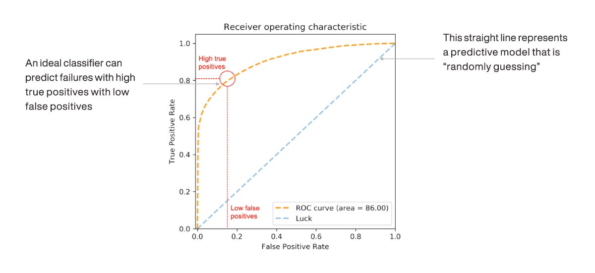
Figure 16 Receiver operating characteristic (ROC) curve
Imagine a classifier starting to make predictions against a finite, labeled data set, while seeking to identify the positive labels within that data set. Before the classifier makes its first prediction, the ROC curve will start at the origin (0, 0). As the classifier starts to make predictions, it sorts them in order of priority – in other words, the predictions the classifier is most “certain” about, with the highest probability of success, are plotted first. A data scientist would hope these initial predictions overwhelmingly consist of positive labels so that there would be many more positive cases surfaced relative to negative ones (TPR should grow faster than FPR). The orange line plotting the performance of the classifier should therefore be expected to grow rapidly from the origin, at a steep slope – as shown in the figure.
At some point, the classifier is unable to distinguish clearly between positive and negative labels, so the number of negative labels surfaced will grow and the number of positive labels remaining will start to dwindle. The classifier performance therefore starts to level off and the FPR starts to grow faster than the TPR. The classifier is forced to surface data points until both TPR and FPR are at 1 – the top right-hand side of the plot.
What is important in this curve is the shape it takes. The start (0,0) and the end (1,1) are pre-determined. It is the initial “steepness” of the curve’s slope and the AUC that matter. As shown in the following figure, the greater the AUC, the better the classifier’s performance.
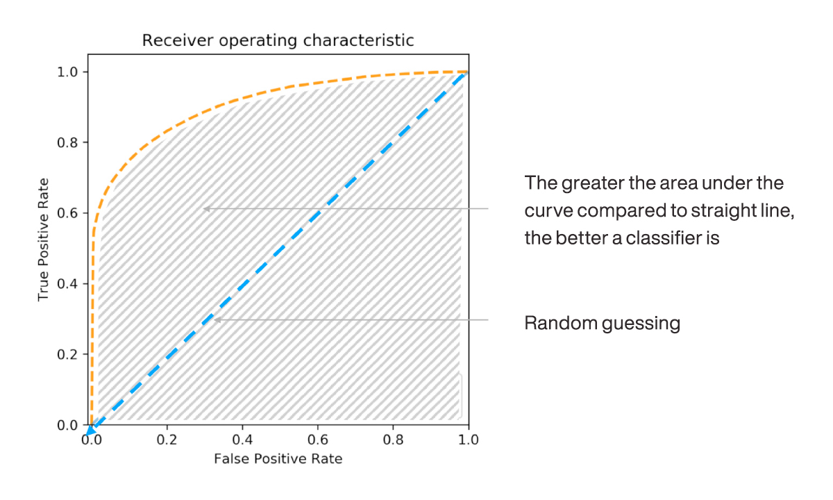
Figure 17 Area under the ROC Curve (AUC) measures how much better a machine learning model predicts classification versus a random luck model.
Note that the classifier’s performance on an ROC curve is compared with random guessing. Random guessing in this case is not a toss of a coin (in other words, a 50 percent probability of getting a class right). Random guessing here refers to a classifier that is truly unable to discern the positive class from the negative class. The predictions of such a classifier will reflect the baseline incidence rates of each class within the data set.
For example, a random classifier used to predict cases of customer attrition will randomly classify customers who are likely to “unsubscribe” with the same incidence rate that is observed in the underlying data set. If the data set includes 100 customers of which 20 unsubscribed and 80 did not, the likelihood of the random classifier making a correct attrition prediction will be 20 percent (20 out of 100).
It can be shown that a random classifier, with predictions that correspond to class incidence rates, will on average plot as a straight line on the ROC curve, connecting the origin to the top right-hand corner.
The AUC of a random classifier is therefore 0.5. Data scientists compare the AUC of their classifiers against the 0.5 AUC of a random classifier to estimate the extent to which their classifier improves on random guessing.
Setting Model Thresholds
A classifier model typically outputs a probability score (between 0 and 1), that reflects the model’s confidence in a specific prediction. While a good starting rule of thumb is that a prediction value greater than 0.5 can be considered a positive case, most real-world use cases require a careful tuning of the classifier value that is determined to be a positive label.
Turning again to the customer attrition example: Should a customer be considered likely to unsubscribe if their score is greater than 0.5 or 0.6, or lower than 0.5? There is no hard-and-fast rule; rather, the actual set point should be tuned based on the specifics of the use case and trade-offs between precision, recall, and specific business requirements. This value that triggers the declaration of a positive label is called the model threshold.
Increasing the model threshold closer to 1 results in a model that is more selective; fewer predictions are declared to be positive cases. Decreasing the threshold closer to 0 makes the model less selective; more predictions are labeled as positives.
The following figure demonstrates how changing the threshold parameter alters the selectivity of a classifier predicting customer attrition. A higher threshold results in higher precision, but lower recall. A lower threshold results in higher recall, but lower precision. It’s therefore important to identify an optimal model threshold with favorable precision and recall.

Figure 18 Threshold selectivity of an ML classifier used to predict customer attrition